INDEX MATCH with multiple criteria

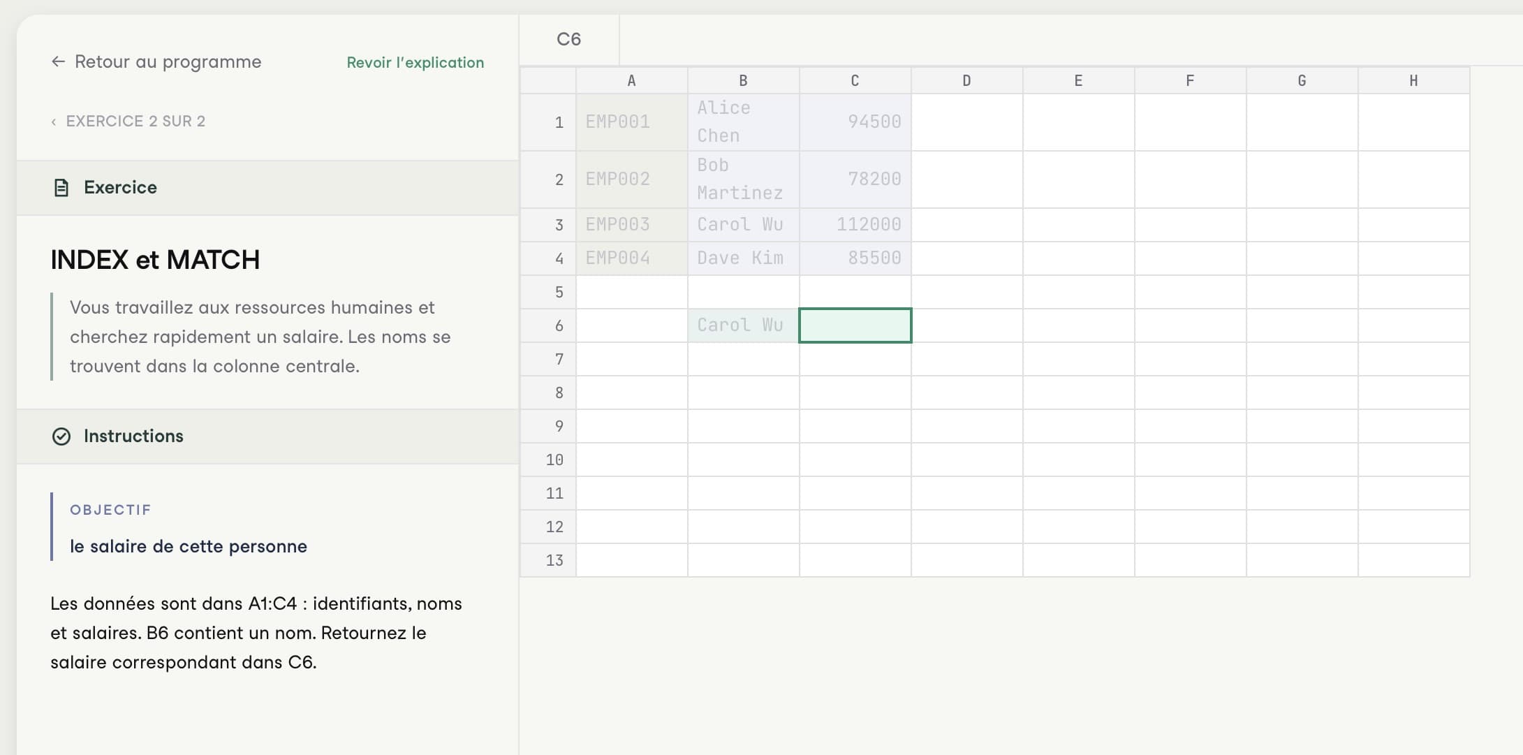
The specific problem

Sometimes a product code is not unique by itself. A price might depend on both SKU and Region, or an employee record might depend on both Name and Department. In those cases, a one-value lookup can return the wrong row.

The classic Excel pattern is `INDEX` with `MATCH` on a combined Boolean test:

=INDEX(return_range, MATCH(1, (sku_range=sku)*(region_range=region), 0))

How to read it

Each comparison returns TRUE or FALSE for every row. Multiplying the comparisons turns rows into 1 only when all criteria are true. `MATCH(1, ..., 0)` finds the first row where every condition matches, and `INDEX` returns the value from the same position.

Common mistakes

• Returning from a range that is a different height than the criteria ranges.
• Forgetting exact match with the final `0` in `MATCH`.
• Using text criteria with hidden spaces, then assuming the lookup formula is broken.
• Expecting this formula to return every match. It returns the first matching row.

When to use XLOOKUP instead

`XLOOKUP` can use the same Boolean technique:

=XLOOKUP(1, (sku_range=sku)*(region_range=region), return_range)

That is often easier to read. `INDEX MATCH` is still useful because it teaches the underlying idea: create a matching position, then return from another range.

Performance notes

Avoid whole-column Boolean array lookups in very large workbooks. Use bounded ranges or Excel Tables. If the lookup runs thousands of times, a helper key such as `SKU&"|"&Region` can make the sheet easier to maintain.

Practice this skill in Calcu

Calcu lookup exercises are designed around the same decision: what uniquely identifies the row, and what range should return the answer?

Related formulas: `XLOOKUP`, `FILTER`, `XMATCH`, `CHOOSECOLS`.